Generate synthetic data with Blender and Python
This blogpost will go through a very attractive alternative for gathering data for a given specific application. Regardless of the type of application, this blogpost seeks to show the reader the pontential of synthetic data generation with open-source resources such as Blender.
Indeed, the need to gather data and label it in a short amount of time is one that hasn’t been exactly solved when it comes to real-life data. This is why, to tackle this problem, we must turn to synthetic data generation which, with the right amount of code, can provide both the labels and the features needed to train a deep learning model later on.
In this case, we focus on an object recognition problem, and we generate the data using Blender and its scripting functionality.
This blogpost is divided into the following main sections:
- 1. Overview of the Project
- 2. Blender scene setup
- 3. Blender scritping
- 4. Test with YOLO and Google Colab
1. Overview of the Project
For this project we are going to generate the data to recognize the wooden toys shown in the images below. In order to do this, we are going to create an algorithm that takes pictures of all of the objects in the same configuration as in the pictures, and also outputs the labels corresponding to the bounding boxes of the location of each object in each image.
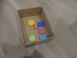
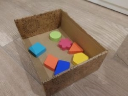
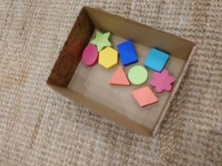
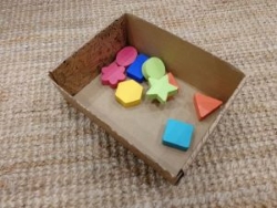
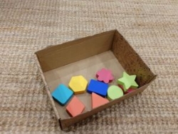
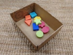
The classes we wish to recognize are the following:
    Pink flower
    Blue square
    Green star
    Yellow hexagon
    Orange lozenge
    Pink oval
    Blue rectangle
    Green circle
    Orange triangle
The algorithm mentioned above is going to be implemented in Python in the rendering software Blender. Blender is an open source software used for multiple rendering applications ranging from animation to product design. This software is going to allows to create realistic renderings of the objects seen above, while allowing us to access the position of each object too, a key feature for the labelling to be done.
The Blender file explained in this blogpost, as well as the entire code and all necessary ressources can be found here.
2. Blender scene setup
Whichever it is the object you want to recognize, in order to generate synth etic data to train its recognizor, we have to represent this or these objects in Blender. Therefore, we have to create and setup a scene that tries to resemble the most to the actual, real-life scene in which we would normally find the objects we want to recognize.
In order to explain how to do this, in this section we’ll walk the reader through the main steps that are necessary to setup a scene that’s compatible with the scripting that will automate the data generation.
Step 1: CAD Model import
The first step consists of importing (or creating) the objects we want to recognize into Blender. In our case, we decided to create the CAD model in Catia V5, and then import it as an .stl. It is also possible to create the model from scratch in Blender, however, as we were more fluent in Catia, we decided to do this on that software.
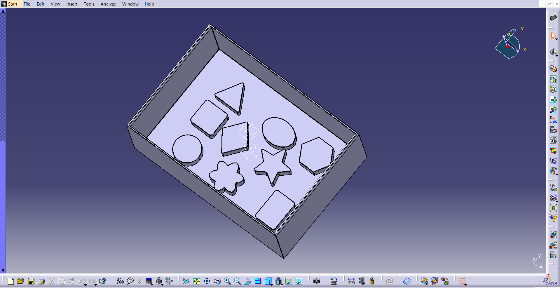 Catia environment with the assembly of the objects we aim to recognize
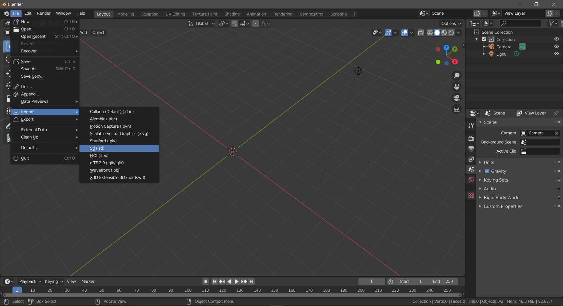
We then move on to opening Blender to start importing each .stl object we want to recognize. We click in the File window, then Import, and finally we select the Stl(.stl) option, in order to import the models previously exported from Catia V5.
 Blender STL file import
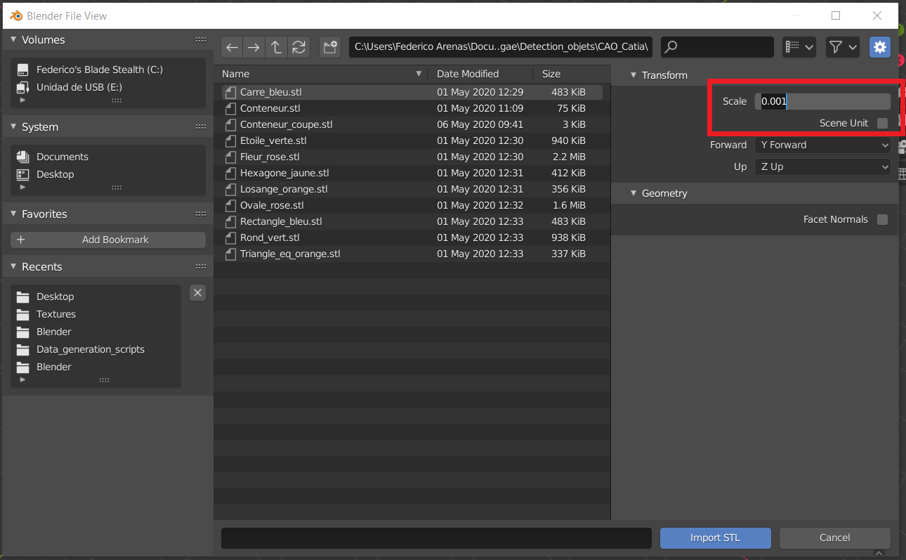
Before finishing the STL import, we have to specify that the scale would be 0.001, since Blender works in meters and Catia works in milimiters. This keeps the units of our model scaled to the Blender reference system, so in later stages the camera has a proportioned size compared to the imported model
 Scaling the STL model before import in Blender
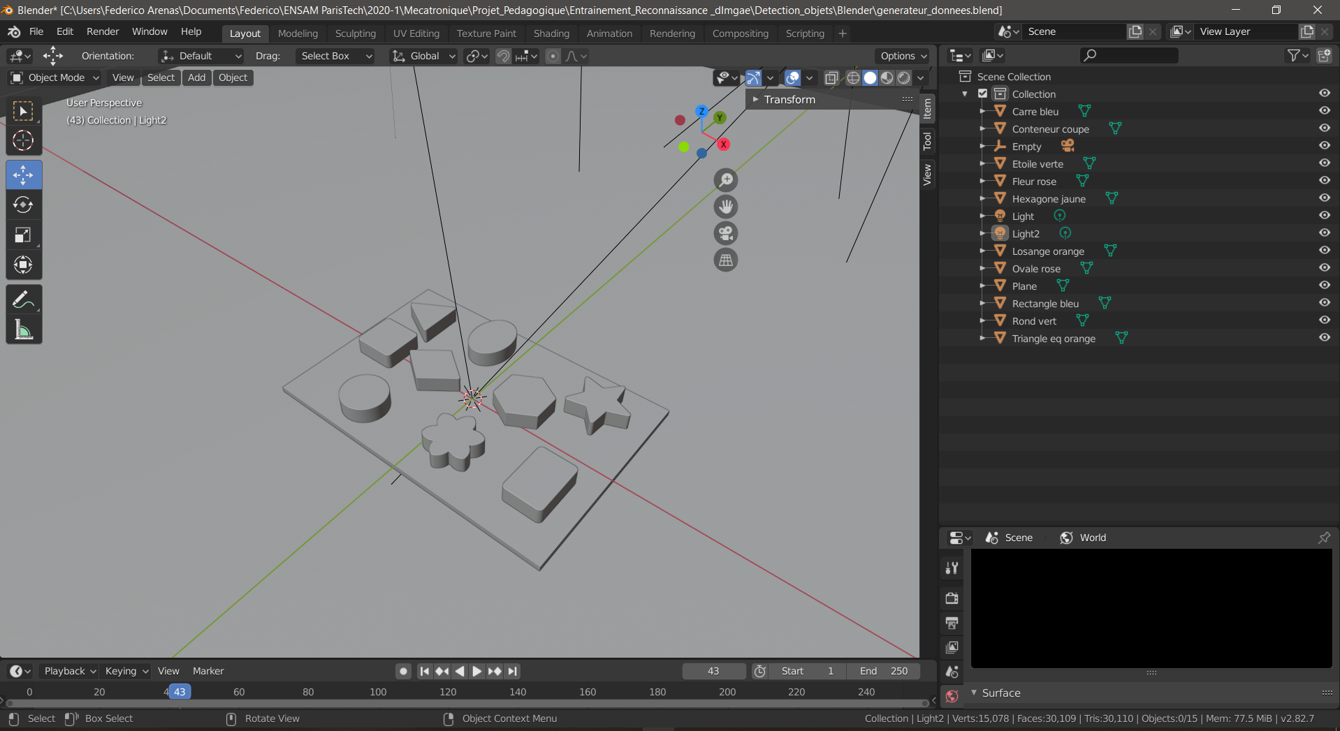
Once each object is imported into the Blender Environment, make sure to create a plane to depict the surface of the scene. Also, make sure to name every object in the Scene Collection menu that can be seen in the right panel in the following image. Make sure these names are easy to write, short and united by an underscore if the name contains two words.
 Final scene with all objects imported and named
Step 2: Scene definition
Once the models are imported, we move onto defning the entiring scene in order to make it look the most realistic. The more realistic the scene is, the better our training data will be, and the better our algorithm will recognize the real-life objects we are training it to detect.
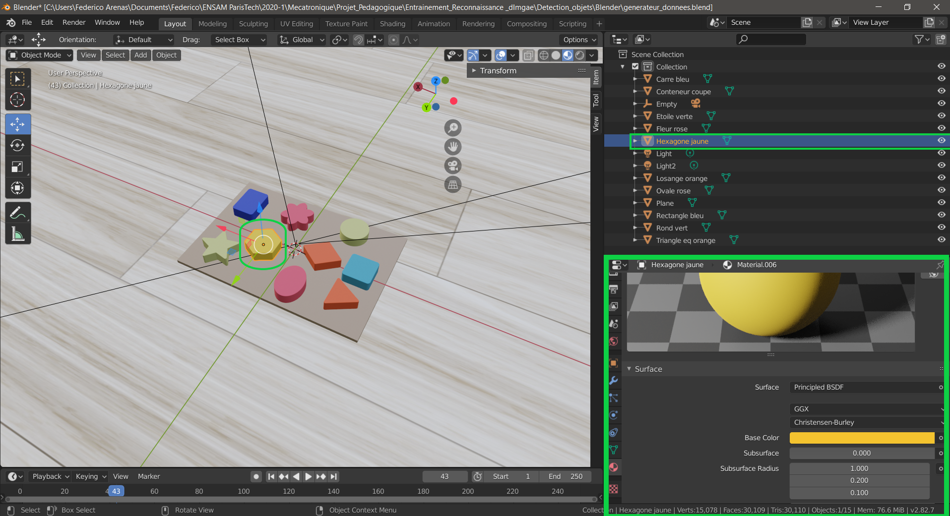
Therefore, we start by defining the materials of each object by selecting it and going into the Material option in the right panel shown below. The three parameters that are key to tuning the appearance of your object are the Base Color, Specular, and Rougness. The las two need to be adjusted to define whether the object absorbs or reflects light, if it is shiny or matte.
 Blender object material definition Panel
Additionnaly, and if necessary, textures can be added to the objects in the scene. These textures can be imported from an image and impose the Base Color from the image. For our project, textures were added to the floor and the platform that holds the objects. A detailed guide on importing textures into Blender can be found here.
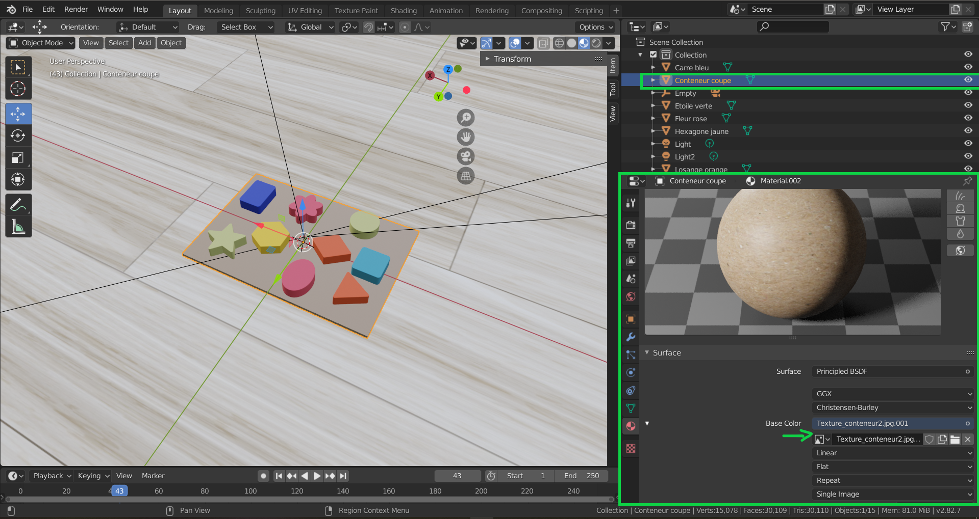 Assigning textures to a Blender object
Next, the lights were defined, the second light can be created by copying and pasting the first light, that is created automatically when the Blender scene is started. As for with the objects, make sure to assign names to these lights such as light1 and light2 that will allow you to call them easily in the code, once we get to the scripting part.
These two lights’ most important parameter is the Power parameter, which will allow us to play with the intensity of the light once we get to the scripting part. In the following picture, on the right bottom part, we can see the “Light Properties” panel being open, with the Power parameter on 16W.
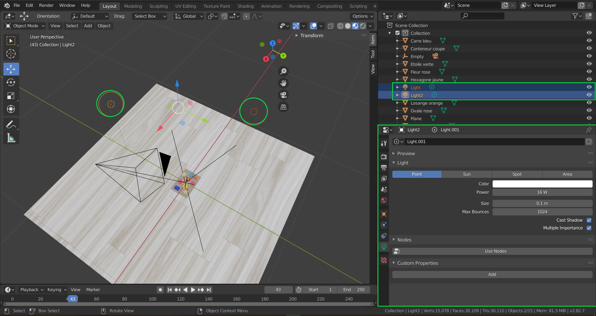 Blender scene with its respective lights
Once all the materials are defined, and the lights that fit your purposes are added, we can move on to visualizing the Rendering by clicking on the top right botton circled in green in the following picture. This allows us to access the Viewport Shading in Rendered mode.
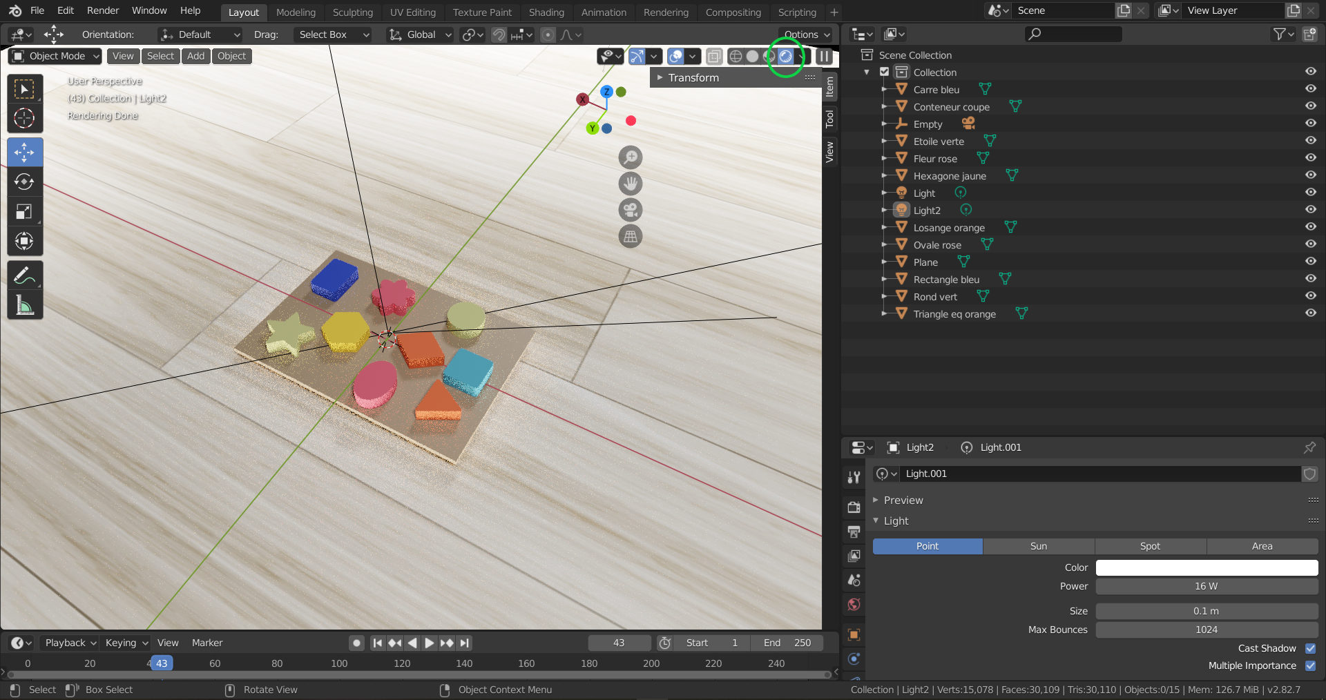 Rendered objects
Now the scene is setup! If any difficulties were found while going through this step, we encourage you to look at a complete guide made by Blender Guru on how to set the rendering configurations in Blender as well as the guide on setting the materials of each object in the scene.
Step 3: Camera setting
The final step to setting up the Blender scene in order to start scripting is setting up the camera! This step is actually crucial because we need to be able to easily control the camera with the scripting in order to make it move around and take pictures. We decided to make the camera orbit all around the objects to take pictures from each angle.
However, this movement isn’t so evident if we think of the cubical space (x,y,z) the camera is set to move on. This means that it would be too complicated to set define a list of (x,y,z) points that describe a spherical movement around the objects. So, in order to simplify this task, we decided to create an axis fixed to the center of the scene, to which the camera would obey when it was moved. This means that when the axis is rotated in the center, the camera will rotate with it. Imagine putting your elbow in a table and moving your fist arond, the fist revolves around your elbow. Now imagine that the elbow is the axis and your fist is the camera, the camera revolves around the axis.
Consequently, we create an axis and locate it in the center of the scene, as shown below.
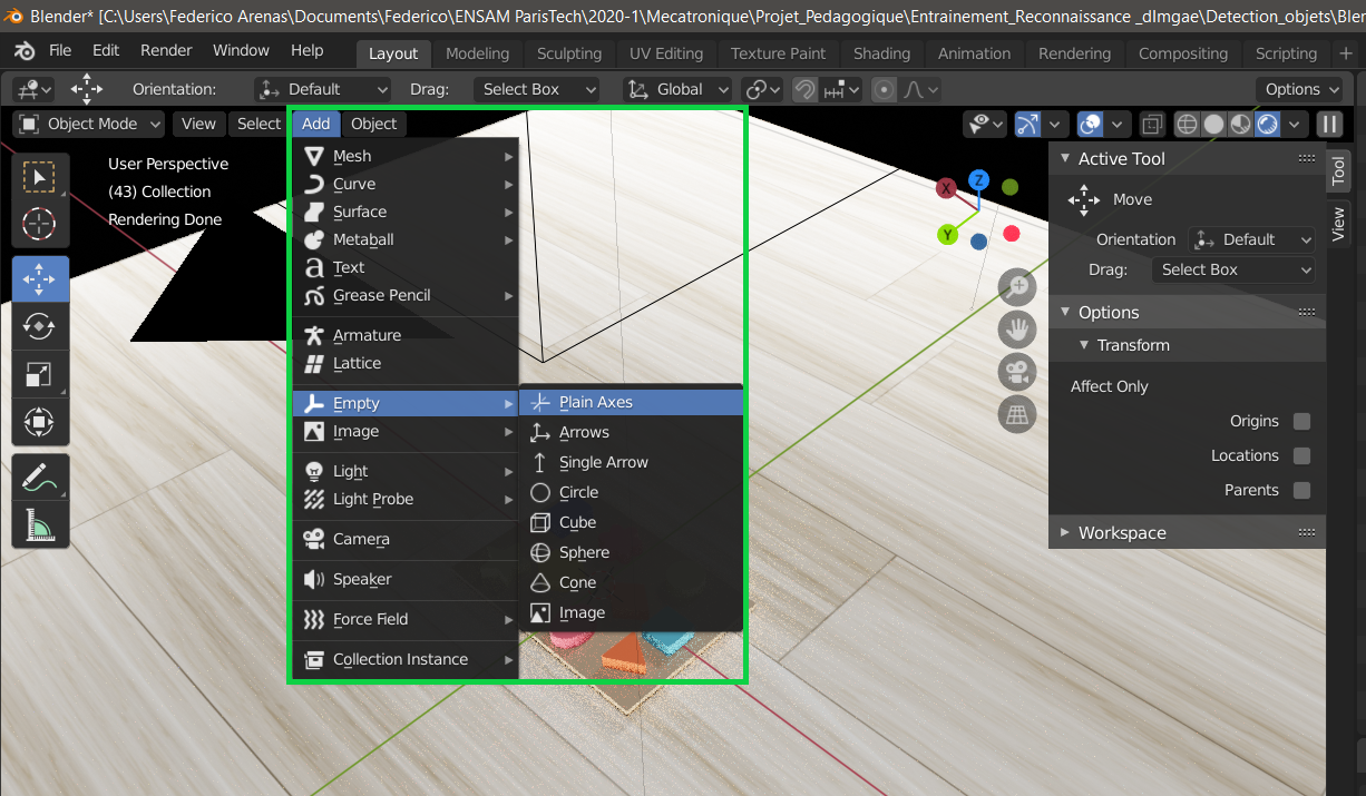 Adding an axis to the center of the scene in Blender
Now, in order to subordinate the movement of the camera to the movement of the axis, we hold Shift and select the camera first and then the axis. Once both of them are selected, hwe hit Ctr + P and select Object (Keep Transform). This will make the axis a parent of the Camera.
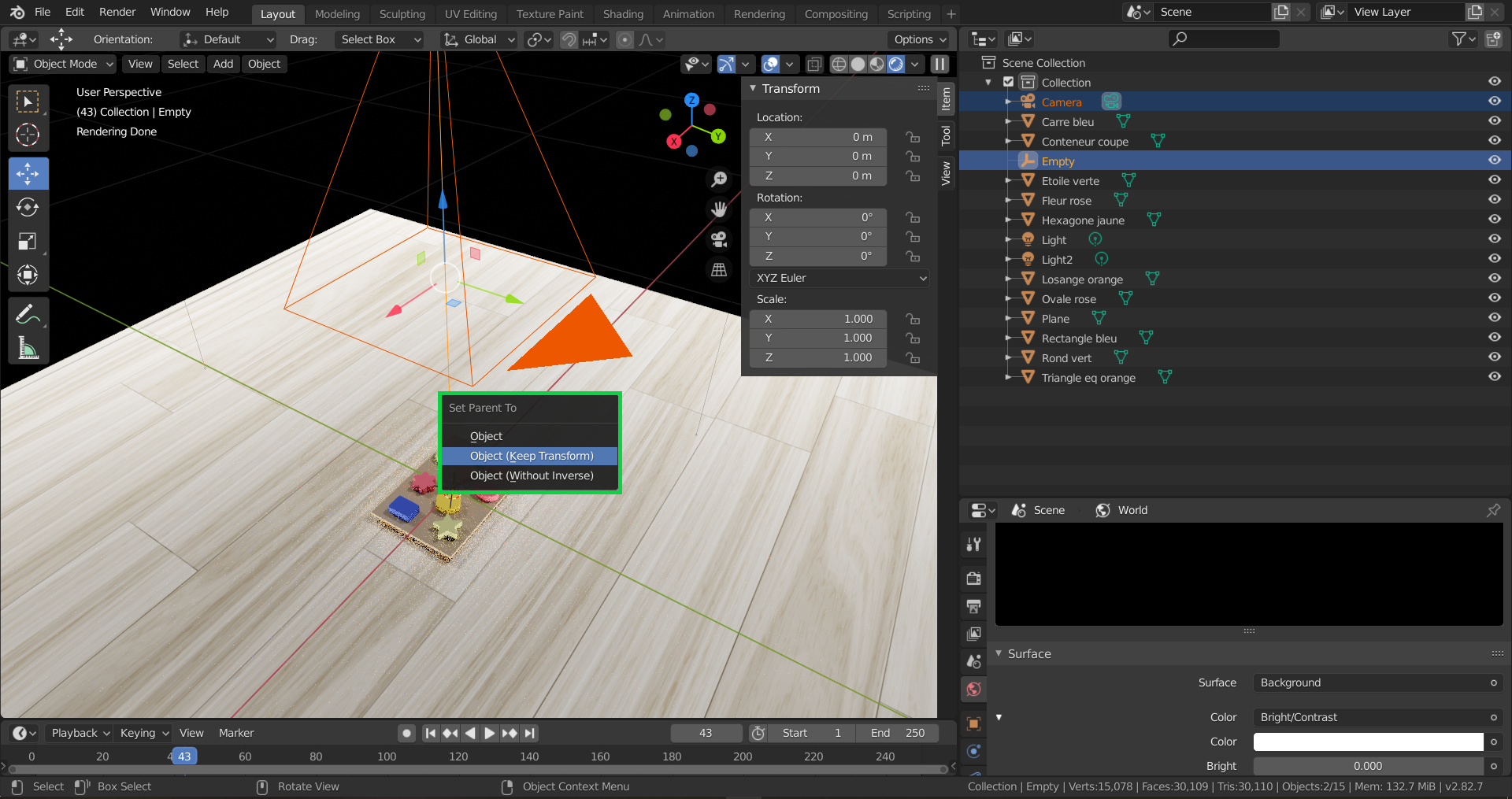 Set the Axis as a Parent of the Camera
You can go ahead and test that this worked by going into Camera view, selecting the axis and going into the Transform window highlighted in green in the image below, and changing the Rotation coordinates of the axis. You’ll see that the camera orbits the objects when the axis rotational coordinates are changed.
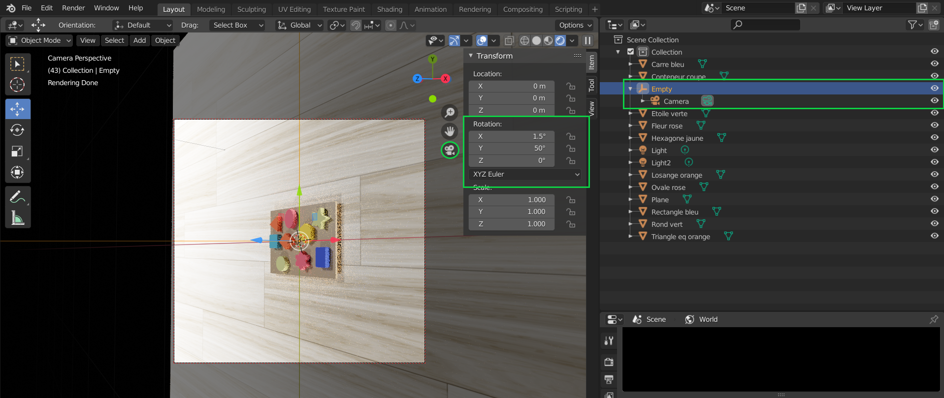 Demonstration of the camera orbiting the objects
Finally, he complete guide to how to set the camera to orbit around a specific object can be found here.
3. Blender scritping
Now that the complete scene is setup, we can start with the scripting. This Blender functionality will allow us to automate the render generation in order to make tens of thousands of pictures and labels that will serve as training data for our object recognition algorithm. This is extremely powerful because this means that if we have a realist-enough Blender scene, we can generate up to 20000 images and labels in around two days (this time will vary according to the capacities of the GPU of your own machine).
This scripting functionality can be accessed by clicking in the Scrpting window underlined in orange in the following picture. By clicking on this window, we-ll have three major elements come up: the Blender Console shown in yellow, the Scripting environment shown in orange, and the Command tracker shown in green.
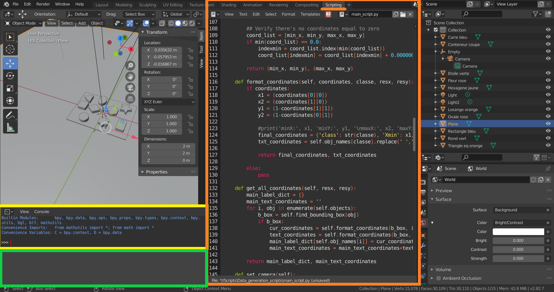 Scripting window and its main components
The Command Tracker allows you to track what actual scripting commands are being used when modifying a specific parameter in the Blender environment. For example, in the following picture I modifyied the position of the Axis.
![]()
Tracking of the script used to change the position of the axis
The Scripting environment allows you to import and save previously created Python Scripts. The script in the Scripting environment will be saved to an external location of your choise. Additionnally, when the script is ready, you can run it by clicking on the Run Script Button
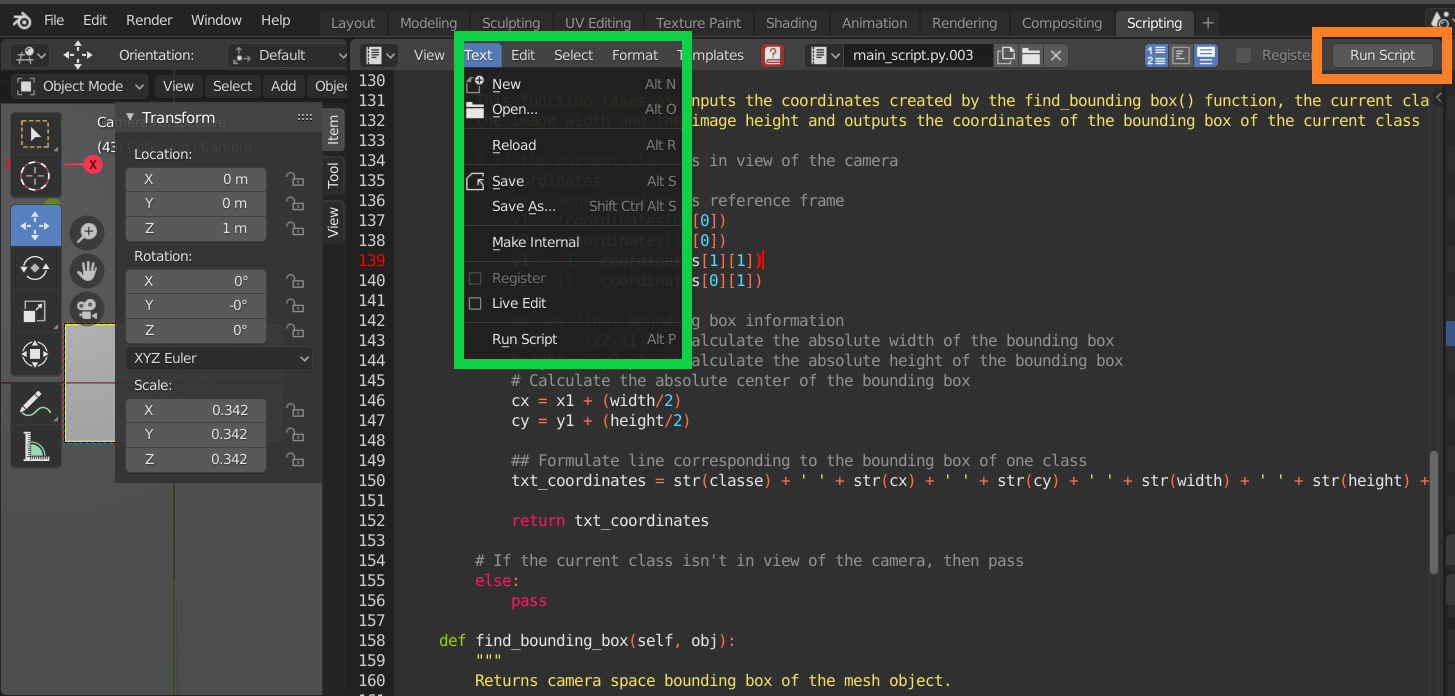 Saving, Opening and Running your script in Blender
Finally, once the script is ready to run, go to Window/Toggle System Console to access the Console that shows the output of your code. This can be better represented in the following image.
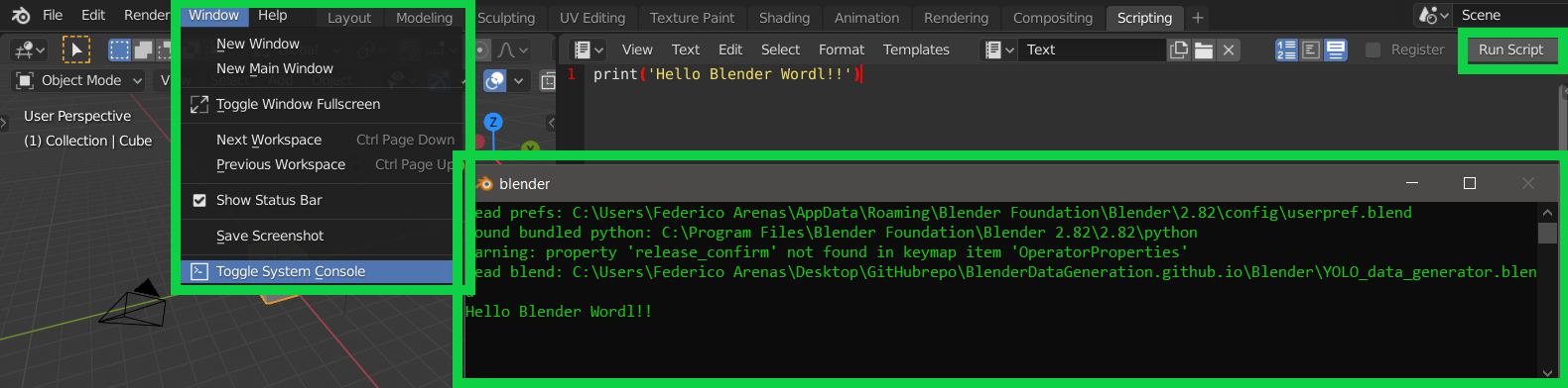 Toggle System Console Output
Introduction to the Blender Console
The Blender Console allows users to enter algorithms into Blender’s environment, using Pyhton language. It is very useful when it comes to generate data automatically. Here we explain the different steps we used to generate our data.
» Accesing scene information
In the following code, you can see how to access to the scene information. bpy.data.scenes is a collection of all the scenes opened in Blender. In our case, only one scene was created. You can access it with the command bpy.data.scenes[0] or bpy.data.scenes[‘Scene’].
>>> bpy.data
<bpy_struct, BlendData at 0x000001C251997458>

>>> bpy.data.scenes
<bpy_collection[1], BlendDataScenes>

>>> bpy.data.scenes[0]
bpy.data.scenes['Scene']

>>> bpy.data.scenes[1]
Traceback (most recent call last):
  File "<blender_console>", line 1, in <module>
IndexError: bpy_prop_collection[index]: index 1 out of range, size 1

>>> scene = bpy.data.scenes[0]
>>> scene
bpy.data.scenes['Scene']
» Accesing object information
We also need to access to the objects information. In fact, we will modifiy several object parameters such as the brightness of the light and the position of the camera. bpy.data.objects is a collection of all the objects of the scene. In our case, we have 15 different objects. Hence, you can call an object from two different ways:
- either you can use the syntax bpy.data.objects[x] where x is a number between 0 and 15 (the amount of objects in the scene)
- or you can use the syntax _bpy.data.objects[‘Name’] where Name is the name of the object you want to call.
You can then store the object you just call in a variable for further use.
>>> bpy.data.objects
<bpy_collection[15], BlendDataObjects>

>>> bpy.data.objects[0]
bpy.data.objects['Camera']

>>> camera = bpy.data.objects['Camera']
>>> bpy.data.objects[1]
bpy.data.objects['Carre bleu']

>>> bpy.data.objects[2]
bpy.data.objects['Conteneur coupe']

>>> bpy.data.objects[3]
bpy.data.objects['Empty']

>>> axe = bpy.data.objects[3]
>>> axe
bpy.data.objects['Empty']

>>> camera
bpy.data.objects['Camera']

>>> carre_bleu = bpy.data.objects['Carre bleu']
>>> carre_bleu
bpy.data.objects['Carre bleu']

>>> bpy.data.objects['Light']
bpy.data.objects['Light']

>>> light1 = bpy.data.objects['Light']
>>> light2 = bpy.data.objects['Light2']
>>> light1
bpy.data.objects['Light']

>>> light2
bpy.data.objects['Light2']
» Modifying object information
For each object, you can modify their information (position, location, etc…) in the scene editor. In the following picture, you can see how to modify the rotation of an object. It is important to understand the utility of the objects’ parameters to be able to create an appropriate algorithm. You can see that when you modify a parameter, its value is updated in the console as well.
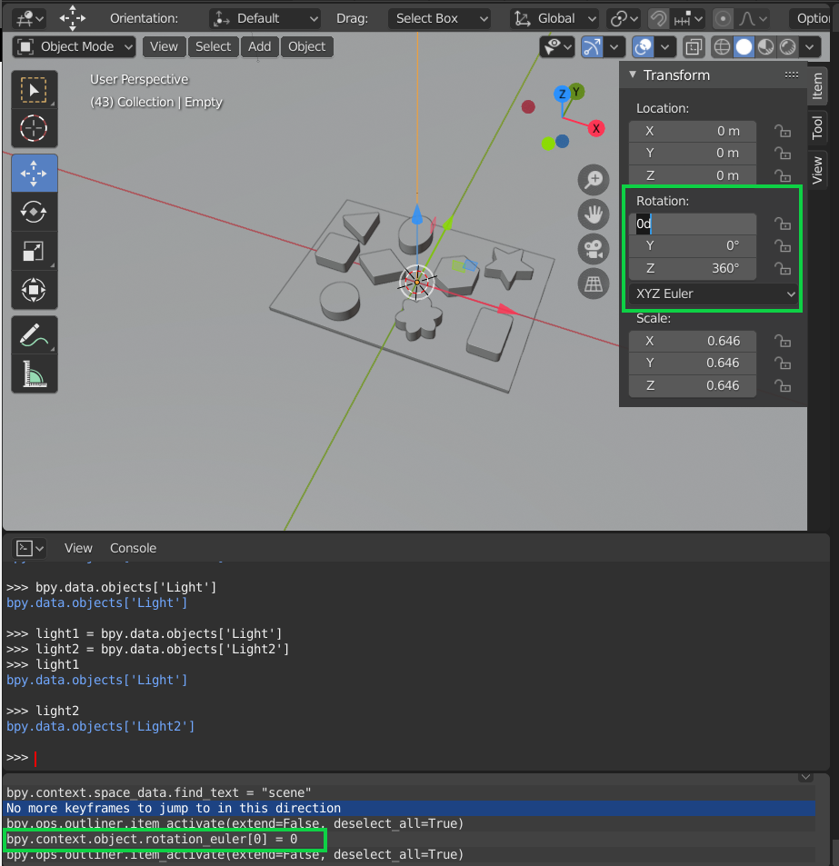 Modifying an object’s parameter
We can now modify the different parameters in the console using the following lines of code:
>>> axe.rotation_euler = (0,0,0)
>>> camera.location = (0,0,0.5)
>>> light1.data.energy = 50
>>> light2.data.energy = 0
light1.data.energy allows you to modify the brightness of the light. camera.location modifies the location of the camera. axe.rotation_euler modifies the rotation of the object ‘axe’.
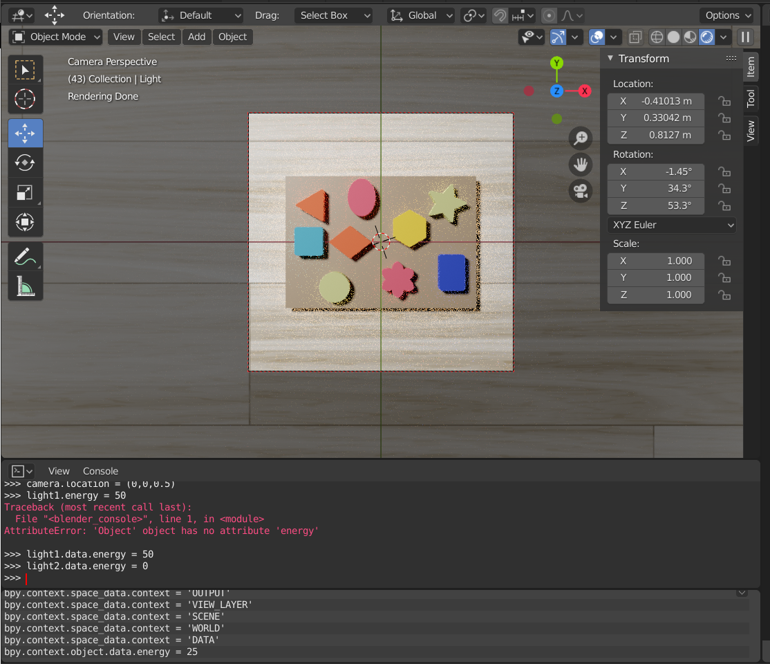 Scene obtained after running the previous lines of code
You can now modify one of the parameter to see how the scene changes.
>>> axe.rotation_euler = (0,0,50)
Here we modified the orientation of the object ‘axe’.
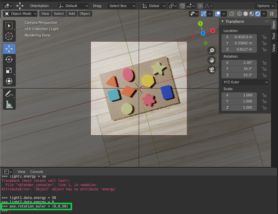 Scene obtained after the modification of the parameter
Main procedure to generate the training data
To train our algorithm, we need a large amount of data. Thus, we will create an algorithm that takes pictures of our objects from different angles by moving the camera around the scene. We will also modify the brightness of the lights in order to obtain a data set more representative of reality.
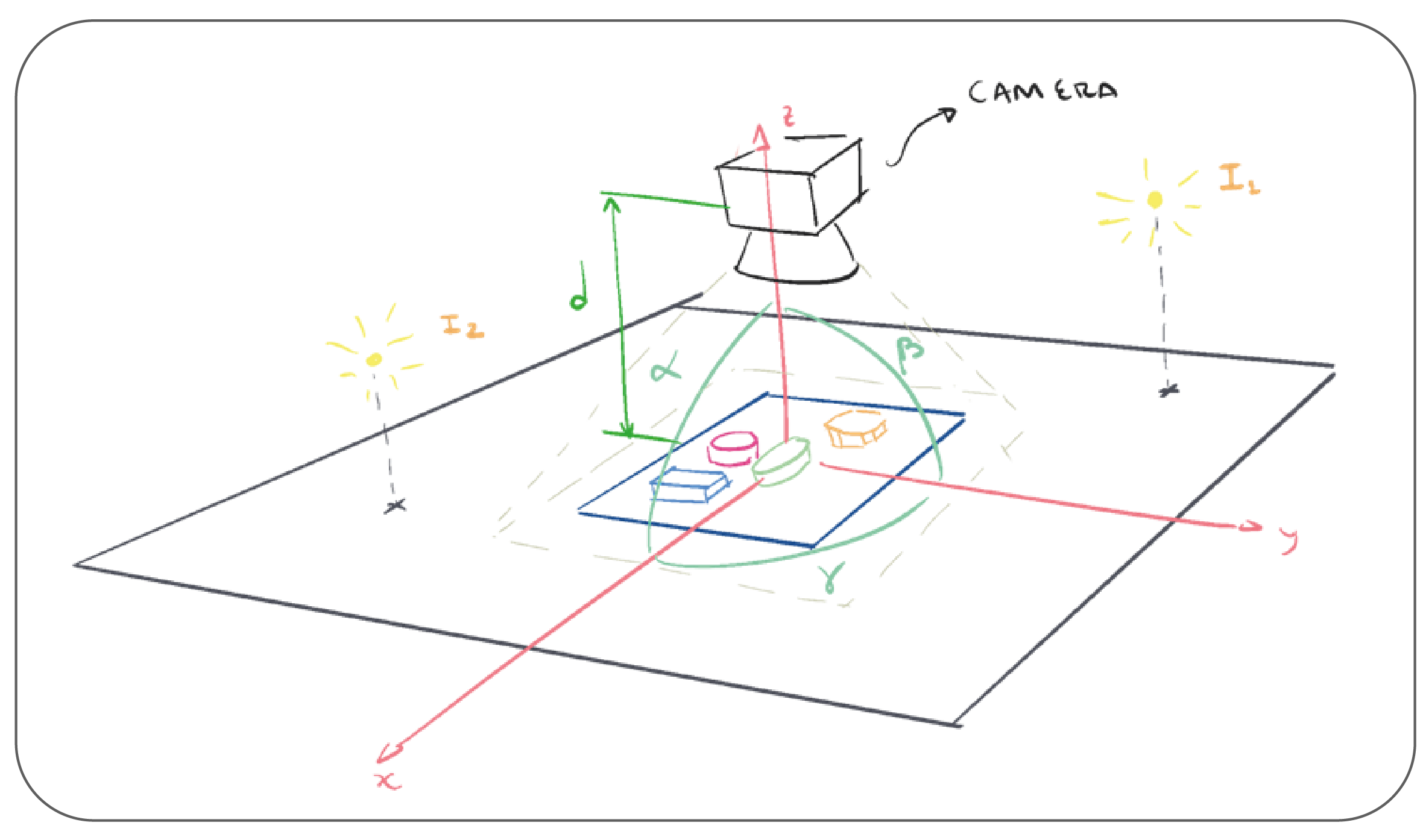 Figure of the environment used in Blender
The following algorithm consists in three loops, each of them modifies one of the angle of the camera (see the previous picture). Inside the loops, we also modify the lights’ brightness. Then, for each position of the camera, we take a picture of the scene and create a text file containing the object information.
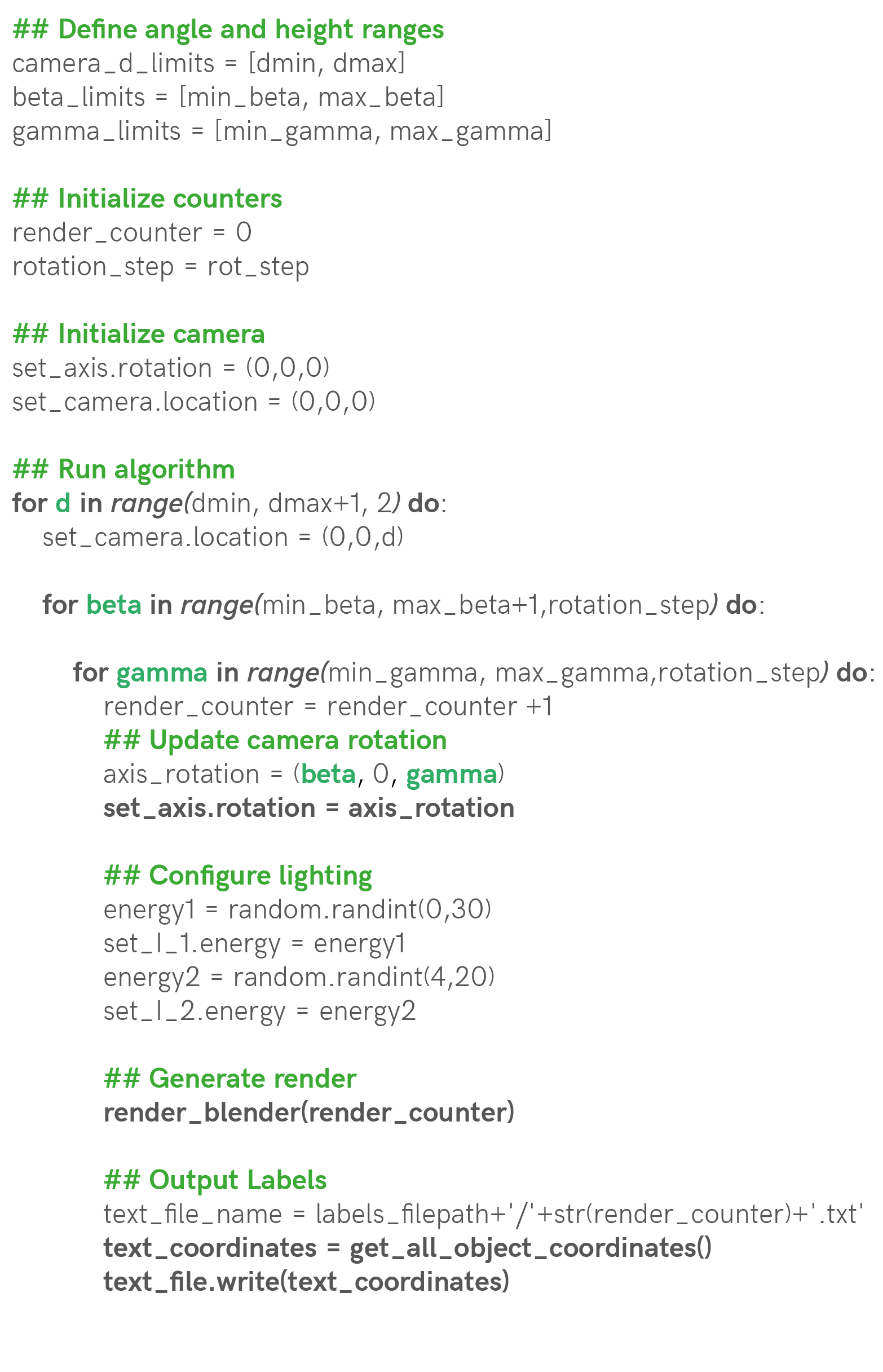
Procedure to generate pictures of the objects
Here you can see pictures taken by the previous algorithm:
Thanks to this algorithm, we will obtain several images with a matching text file containing the location of the objects and their bounding box. This data set will then be used to train a deep learning algorithm.
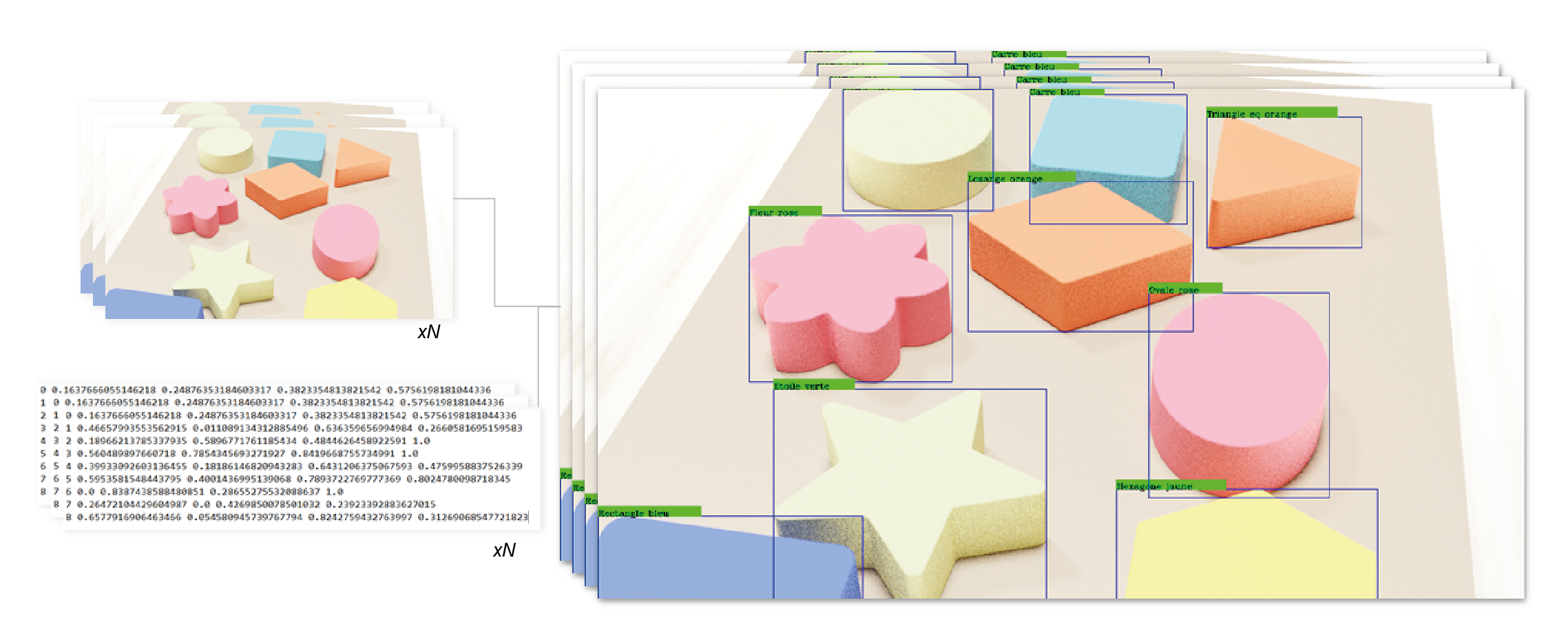 Expected results of the algorithm
Rendering class initial definition
In order to implement a program that incorporates the algorithm explained above and is able to access the information of the Scene and the Objects in it, we have decided to create an entire class named Render.
This class is initialized below. We begin by importing all the relevant libraries. bpy is the library that allows us to access and modify the information of the Blender elements. During the initialization of the Render class, we define the main objects that we will be manipulating such as the camera defined as self.camera, the axis defined as self.axis, the light 1 and 2 defined as self.light1 and self.light2, and all the objects that are saved into the self.objects variable.
Finally, but most immportantly, we define the variable self.camera_z_limits to move the camera from 0.3 meters to 1 meter, each 0.1 meters. We define the self.beta_limits to rotate the camera along the x axis from 80º to -80º, each rot_step angles. We define the self.gamma_limits to rotate the camera along the x axis from 0º to 360º, each rot_step angles. Also, we define the self.images_filepath and self.labels_filepath which will be the filepaths were the images and labels generated by our program will be saved.
## Import all relevant libraries
import bpy
import numpy as np
import math as m
import random

## Main Class
class Render:
    def __init__(self):
        ## Scene information
        # Define the scene information
        self.scene = bpy.data.scenes['Scene']
        # Define the information relevant to the <bpy.data.objects>
        self.camera = bpy.data.objects['Camera']
        self.axis = bpy.data.objects['Main Axis']
        self.light_1 = bpy.data.objects['Light1']
        self.light_2 = bpy.data.objects['Light2']
        self.obj_names = ['Rose Flower', 'Blue Square', 'Green star', 'Yellow hexagon', 'Orange losange',
                          'Rose oval', 'Blue rectangle', 'Green circle', 'Orange triangle']
        self.objects = self.create_objects() # Create list of bpy.data.objects from bpy.data.objects[1] to bpy.data.objects[N]

        ## Render information
        self.camera_d_limits = [0.2, 0.8] # Define range of heights z in m that the camera is going to pan through
        self.beta_limits = [80, -80] # Define range of beta angles that the camera is going to pan through
        self.gamma_limits = [0, 360] # Define range of gamma angles that the camera is going to pan through

        ## Output information
        # Input your own preferred location for the images and labels
        self.images_filepath = 'C:/Users/Federico Arenas/Desktop/Webinar/Tutorial Blender/Blender/Data'
        self.labels_filepath = 'C:/Users/Federico Arenas/Desktop/Webinar/Tutorial Blender/Blender/Data/Labels'

    def set_camera(self):
        self.axis.rotation_euler = (0, 0, 0)
        self.axis.location = (0, 0, 0)
        self.camera.location = (0, 0, 3)
Main algorithm to pan around the objects and take pictures
Now, we’ll add the main_rendering_loop() function to the Render class. This function is the implementation in Python of the algorithm shown in the previous section. By acessing the self.camera, self.axis, self.light1, and self.light2 information we’ll be able to move the camera around the objects, take the pictures and extract the labels.
Initially, by using the self.calculate_n_renders(rot_step) function, we are able to calculate how many renders and labels will be created. The rot_step parameter indicates each how many degrees the program is going to take a picture. The smaller rot_step is, the more renders and labels will be created. We then print the information of the number of renders, and ask whether to start the rendering or not. This is important because it allows us to estimate what rot_step is going to give us how many renders, if its too many, we increase the rot_step, if it’s too little, we reduce it.
If the user hits ‘Y’ then the algorithm starts creating the data. It must be noted that we have to do some refactoring and adapt the initially defined limits self.camera_z_limits, self.beta_limits, and self.gamma_limits. This refactoring is done because the for loop can’t loop through decimal numbers nor through negative numbers, so we’re forced to multiply by ten for the decimals, and use 10º to 170º, instead of 80º to -80º.
    def main_rendering_loop(self, rot_step):
        '''
        This function represent the main algorithm explained in the Tutorial, it accepts the
        rotation step as input, and outputs the images and the labels to the above specified locations.
        '''
        ## Calculate the number of images and labels to generate
        n_renders = self.calculate_n_renders(rot_step) # Calculate number of images
        print('Number of renders to create:', n_renders)

        accept_render = input('\nContinue?[Y/N]:  ') # Ask whether to procede with the data generation

        if accept_render == 'Y': # If the user inputs 'Y' then procede with the data generation
            # Create .txt file that record the progress of the data generation
            report_file_path = self.labels_filepath + '/progress_report.txt'
            report = open(report_file_path, 'w')
            # Multiply the limits by 10 to adapt to the for loop
            dmin = int(self.camera_d_limits[0] * 10)
            dmax = int(self.camera_d_limits[1] * 10)
            # Define a counter to name each .png and .txt files that are outputted
            render_counter = 0
            # Define the step with which the pictures are going to be taken
            rotation_step = rot_step

            # Begin nested loops
            for d in range(dmin, dmax + 1, 2): # Loop to vary the height of the camera
                ## Update the height of the camera
                self.camera.location = (0, 0, d/10) # Divide the distance z by 10 to re-factor current height

                # Refactor the beta limits for them to be in a range from 0 to 360 to adapt the limits to the for loop
                min_beta = (-1)*self.beta_limits[0] + 90
                max_beta = (-1)*self.beta_limits[1] + 90

                for beta in range(min_beta, max_beta + 1, rotation_step): # Loop to vary the angle beta
                    beta_r = (-1)*beta + 90 # Re-factor the current beta

                    for gamma in range(self.gamma_limits[0], self.gamma_limits[1] + 1, rotation_step): # Loop to vary the angle gamma
                        render_counter += 1 # Update counter

                        ## Update the rotation of the axis
                        axis_rotation = (m.radians(beta_r), 0, m.radians(gamma))
                        self.axis.rotation_euler = axis_rotation # Assign rotation to <bpy.data.objects['Empty']> object
                        # Display demo information - Location of the camera
                        print("On render:", render_counter)
                        print("--> Location of the camera:")
                        print("     d:", d/10, "m")
                        print("     Beta:", str(beta_r)+" Deg")
                        print("     Gamma:", str(gamma)+" Deg")

                        ## Configure lighting
                        energy1 = random.randint(0, 30) # Grab random light intensity
                        self.light_1.data.energy = energy1 # Update the <bpy.data.objects['Light']> energy information
                        energy2 = random.randint(4, 20) # Grab random light intensity
                        self.light_2.data.energy = energy2 # Update the <bpy.data.objects['Light2']> energy information

                        ## Generate render
                        self.render_blender(render_counter) # Take photo of current scene and ouput the render_counter.png file
                        # Display demo information - Photo information
                        print("--> Picture information:")
                        print("     Resolution:", (self.xpix*self.percentage, self.ypix*self.percentage))
                        print("     Rendering samples:", self.samples)

                        ## Output Labels
                        text_file_name = self.labels_filepath + '/' + str(render_counter) + '.txt' # Create label file name
                        text_file = open(text_file_name, 'w+') # Open .txt file of the label
                        # Get formatted coordinates of the bounding boxes of all the objects in the scene
                        # Display demo information - Label construction
                        print("---> Label Construction")
                        text_coordinates = self.get_all_coordinates()
                        splitted_coordinates = text_coordinates.split('\n')[:-1] # Delete last '\n' in coordinates
                        text_file.write('\n'.join(splitted_coordinates)) # Write the coordinates to the text file and output the render_counter.txt file
                        text_file.close() # Close the .txt file corresponding to the label

                        ## Show progress on batch of renders
                        print('Progress =', str(render_counter) + '/' + str(n_renders))
                        report.write('Progress: ' + str(render_counter) + ' Rotation: ' + str(axis_rotation) + ' z_d: ' + str(d / 10) + '\n')

            report.close() # Close the .txt file corresponding to the report

        else: # If the user inputs anything else, then abort the data generation
            print('Aborted rendering operation')
            pass
You might have noticed that we call two functions that are created by us: self.render_blender(render_counter) and self.get_all_coordinates(resx, resy). The first function, which is included in the source code, varies the image size and definition, takes a picture and defines the _self.xpix, self.ypix and self.percentage variables, which are the size of the picture taken and its scale provided in %. This function ultimately exports the render_counter.png file to the self.images_filepath location.
We can see that the resx and resy are take these variables into account when inputted into the self.get_all_coordinates(resx, resy) function. The following calculation is done to provide the final size of the image:
resx = final x size of the image = self.xpix * self.percentage * 0.01 # Multiply by 0.01 to divide by 100 and scale the final size
resy = final y size of the image = self.ypix * self.percentage * 0.01 # Multiply by 0.01 to divide by 100 and scale the final size
This second function will be further explained in the following section. Once the coordinates a recovered, they are added to the render_counter.txt file created that is saved in the self.labels_filepath location.
Main function to extract labels from all objects in image
The fonction get_all_coordinates(resx, resy) loops through all the objects in self.objects and tries to get each object’s coordinates with the function self.find_bounding_box(obj) which takes the current object obj and if in view of the camera, outputs its coordinates. This function is further explained here, and is integrated into the full code we made here.
Next, if the object is found, the function self.format_coordinates(b_box, i, resx, resy) reformats the labels of each object from this format:
```
Name_of_class_0 <top_x> <top_y> <bottom_x> <bottom_y>
Name_of_class_1 <top_x> <top_y> <bottom_x> <bottom_y>
Name_of_class_2 <top_x> <top_y> <bottom_x> <bottom_y>
...
...
Name_of_class_N <top_x> <top_y> <bottom_x> <bottom_y>
```
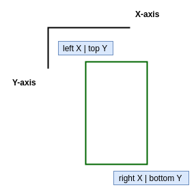
Initial format of the label (source)
to the format used by YOLO:
```
0 <center_x> <center_y> <bounding_box_width> <bounding_box_height>
1 <center_x> <center_y> <bounding_box_width> <bounding_box_height>
2 <center_x> <center_y> <bounding_box_width> <bounding_box_height>
...
...
N_classes <center_x> <center_y> <bounding_box_width> <bounding_box_height>
```
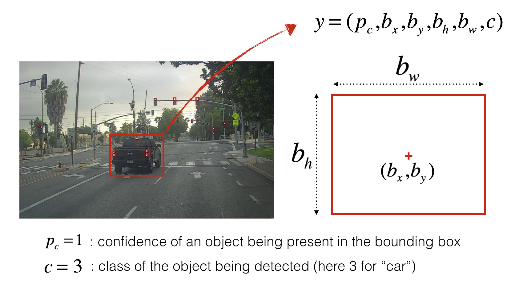
Format of the label after formatting (source)
The function can be seen here:
    def get_all_coordinates(self):
        '''
        This function takes no input and outputs the complete string with the coordinates
        of all the objects in view in the current image
        '''
        main_text_coordinates = '' # Initialize the variable where we'll store the coordinates
        for i, objct in enumerate(self.objects): # Loop through all of the objects
            print("     On object:", objct)
            b_box = self.find_bounding_box(objct) # Get current object's coordinates
            if b_box: # If find_bounding_box() doesn't return None
                print("         Initial coordinates:", b_box)
                text_coordinates = self.format_coordinates(b_box, i) # Reformat coordinates to YOLOv3 format
                print("         YOLO-friendly coordinates:", text_coordinates)
                main_text_coordinates = main_text_coordinates + text_coordinates # Update main_text_coordinates variables whith each
                                                                                 # line corresponding to each class in the frame of the current image
            else:
                print("         Object not visible")
                pass

        return main_text_coordinates # Return all coordinates
Finally, the main_text_coordinates are returned as a string.
Results obtained from the data generation
We run the following code, which calls the Render() class, initializes de camera end then starts the data generation loop.
## Run data generation
if __name__ == '__main__':
    # Initialize rendering class as r
    r = Render()
    # Initialize camera
    r.set_camera()
    # Begin data generation
    rotation_step = 5
    r.main_rendering_loop(rotation_step)
The program will output the progress to the Blender Toggle Console Window. It will output the images and labels to the specified locations.
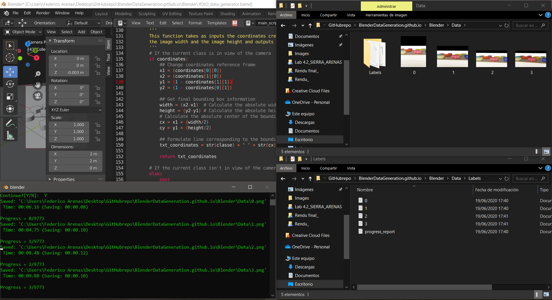 Messages in the Toggle Console Window
The labels, as mentioned before, will have the following format.
```
0 <center_x> <center_y> <bounding_box_width> <bounding_box_height>
1 <center_x> <center_y> <bounding_box_width> <bounding_box_height>
2 <center_x> <center_y> <bounding_box_width> <bounding_box_height>
...
...
N_classes <center_x> <center_y> <bounding_box_width> <bounding_box_height>
```
Finally, we run a program that draws the outputted labels to the outputted images in order to verify that these labels are correctly pointing to each of the objects.
4. Test with YOLO and Google Colab
We decided to use the Darknet architecture using YOLOv3, and implemented in Google Colab. We downloaded the darknet architecture from AlexeyAB’s Darknet repository, and learned how to implement it using this source.
This blogpost focuses on the procedure to automate training data generation for a YOLO application, and not on the training itself, so this section’s purpose is to show a short summary of our results, and is not meant to be explanatory.
Results obtained
We made 5 different tests in order to obtain the best performance. However, we were highly limited by the processing capacities of our own computer, with a GPU Nvidia GeForce MX150, the rendering of around 10000 images would take up to a day and a half. This means that the creation of datasets of around 100000 images would not be feasible, since we would need to use our computer for other purposes too.
In any case, the training outputted the following loss charts.
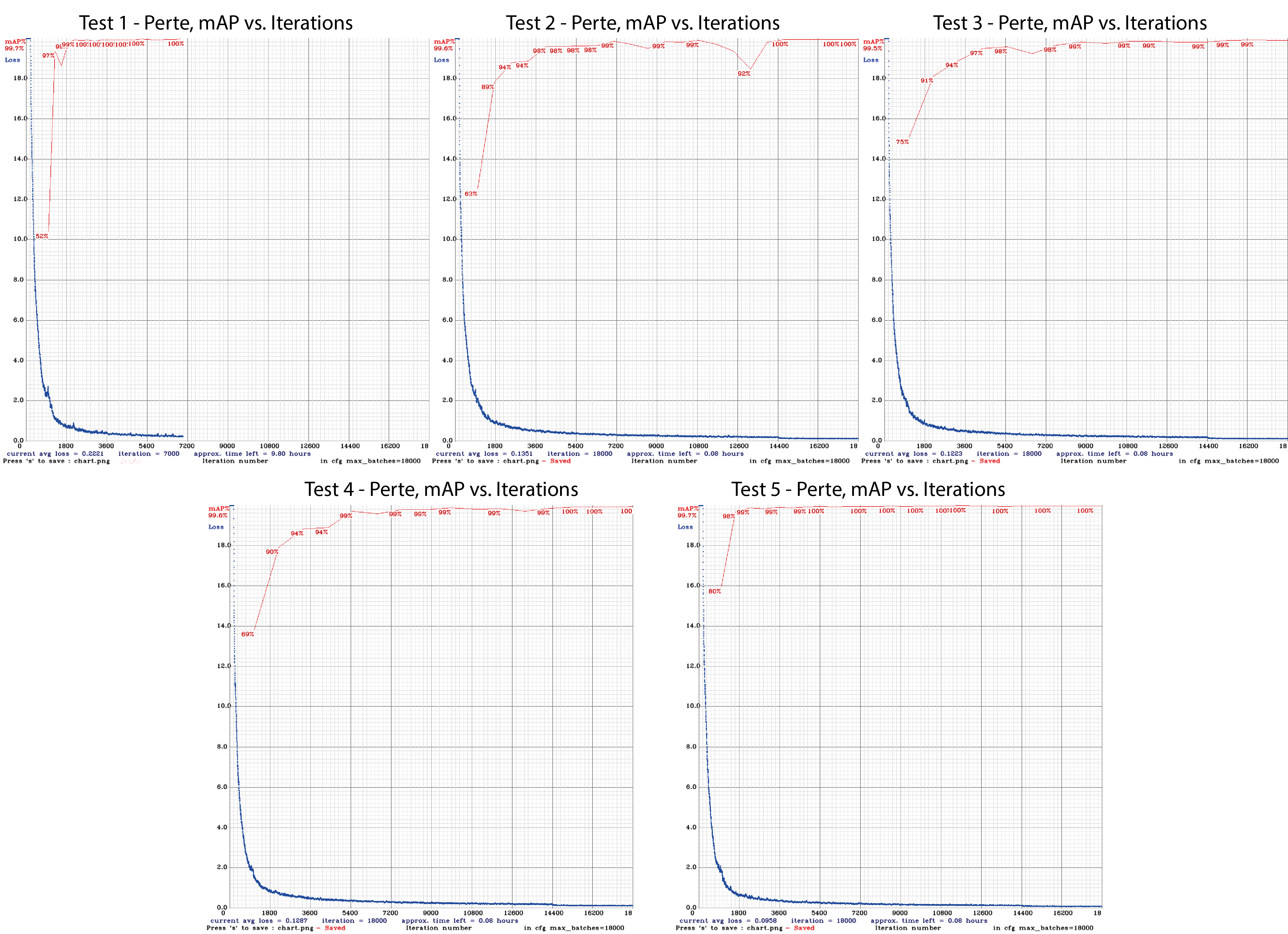
We made a summary of the results and found that increasing the quantity of data isn’t always helpful if you are not representing the variations that the test will contain. This can be seen in the comparison between Test 1 and Test 5.
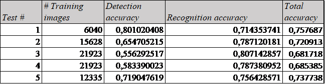
The recognition results are satisfactory taking into account that it took us around a week to obtain the data and train our models, with low-capacity computers. This means that the scalability of synthetic data generation is very good. With better resources, we can train our algorithms with a lot more data, and even more photo-realistic.
A demonstration of the algorithm working on synthetic test data can be seen below and the full video can be found here.
A demonstration of the algorithm working on real test data can be seen below and the full video can be found here.